Basic Theory - Day 1

Introduction to fractals and multifractals

• What are fractals?

  • Highly irregular : fractal objects tend to be highly irregular and fill the space in which it is embedded.

  • Self-similarity : an object that displays the same basic pattern at all scales. The simplest fractals are deterministic, and are generated using recursive or iterative procedures.

  • Fractal Dimension : the characteristic are captured by a dimension that is a measure of complexity of the object.

Ecological fractals

• Fractal behavior can be observed looking at different scales. In the next figure (modified from Solé & Bascompte 2006) a beetle species walks on the surface of a trunk with lichens carrying lichens on its back.

  

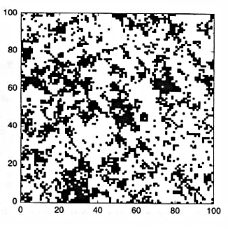
  The spatial distribution of low canopy areas (less than 15m) in a rainforest in Panama (BCI) where clusters of many different sizes can be observed

  

Deterministic fractals

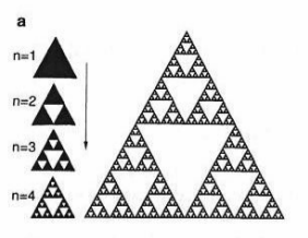
• The Sierpinsky gasket : Starting with an equilateral triangle, the procedure consist on removing from the central portion an upside down equilateral triangle with half the side length of the starting triangle.

  

Deterministic fractals 1

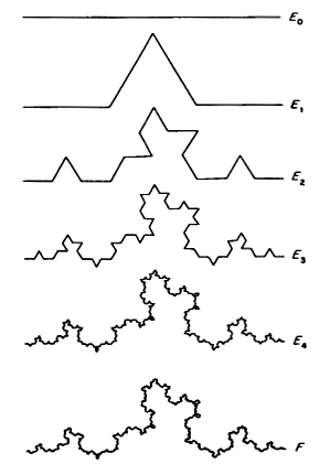
• The Coch curve: A segment of length 1 is divided into thirds. The center one is replaced by the other two sides of an equilateral triangle of length 1/3.

  

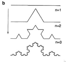
  The curve occupies a definite space, but its length $L$ goes to infinity.

  We can compute $L_n$ at different steps $n$

  $L_0=1$

  $L_1=4/3$

  $L_2=(4/3)^2$

  At an arbitrary step $L_n=(4/3)^n$ that goes to infinity as $n$ grows.

• Why $L_n=(4/3)^n$ ?

Dynamic fractals

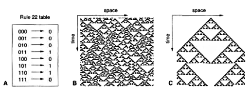
• Cellular automata (CA) are discrete time, discrete space and discrete state dynamical models. We will consider a one dimensional CA with N sites. We can think that each site contains one individual of one species $S_i(t)$ for $i=1,…,N$

• Each time step all elements are updated following a rule table:

  $S_i(t+1) = \Phi \left( S_{i-1}(t),S_{i}(t),S_{i+1}(t) \right)$

  The state of each unit change according to its own state and the state of some neighborhood.

• The simplest case is that we have only one species: the possible states are 0 and 1.

  

Exercise: play with 1D CA

• Rule 22 (monogamy)

    current pattern     111   110    101    100    011    010   001   000  
    -----------------  ----- -----  -----  -----  -----  ----- ----- ----- 
    new state            0     1      1      0      1      0     0     0
  

  Starting with the following initial configurations

    a) 1 0 1 0 1 0 1 0 1 0
  
    b) 0 1 1 0 1 0 1 1 0 0
  

• But the rule 22 does not generate the Sierpinsky triangle, the following rule generates it:

    current pattern    111   110   101   100   011   010   001   000   
    ----------------- ----- ----- ----- ----- ----- ----- ----- ----- 
    new state           0     1     0     1     1     0     1     0     
  

  Starting with the following initial configurations

    a) 0 0 0 0 1 0 0 0 0 0
  

Random Fractals

• All the previous fractals constructions have random analogues. In the Von Koch curve we replace the middle third by the sides of an equilateral triangle, we might toss a coin to determine the position of the new part above or below the removed segment.

  

Statistical self similarity

• The pattern of random fractals is self-similar in the statistical sense.

  • A given property $L(r)$, which can be length, mass, population abundance or number or species, measured at some scale of resolution $r$.

  • Then we look at a different scale $r'=\alpha r$. If $\alpha < 1$ then is a finer resolution, else a coarser resolution.

  • Statistical self similarity means that $L(r)$ is proportional to $L(\alpha r)$

    $L(\alpha r) = k L(r)$

    where k is a constant.

  • This definition implies that the statistical features of a fractal set are the same when measured at different scales.

Scaling laws

• Statistical self similar patterns can be analyzed by power laws or scaling laws

  • Zipf’s law : one of the best known scaling laws

    The fraction of cities $N(n)$ with $n$ inhabitants shows a power law dependence:

    $N(n) \propto n^{-r}$ with $r \approx 2$

  • An example of an ecological scaling law is the frequency distribution of biomass, the plot shows the cumulative distribution $N(>n)$ against biomass

    

    Scaling in the cumulative biomass distribution of all organisms in lake Konstanz (from Gaedke 1992).

    For a scaling law $N(n) \propto n^{-r}$ we get $N(>n) \propto n^{-r+1}$

Power laws are scale invariant

• To show that power laws are scale invariant we can see the effect of a scale transformation.

  Self similarity implies:

  $\frac{L(r)}{L(\alpha r)}=k$

  Let us assume that $L(r)$ follows a power law

  $L(r)=A r^\eta$

  then

  $\frac{A r^\eta}{A (\alpha r)^\eta} = \frac{1}{\alpha^\eta} = k $

Fractal dimension

• Let us consider different geometric objects:

  • A line $\Omega_1$ of length $L$

  • A square $\Omega_2$ of area $L^2$

  • A cube $\Omega_3$ with volume $L^3$

• We want to cover these with a set of identical non-overlaping segments/squares/cubes of side $\epsilon L$ with $\epsilon < 1$.

  The number of segments required to cover $\Omega_1$ will be

  $N(\epsilon) = \frac{L}{\epsilon L} =\epsilon^{-1}$

  For the squares $\frac{L^2}{(\epsilon L)^2} =\epsilon^{-2}$

  In general

  $N(\epsilon) = \epsilon^{-d}$

  Where $d=dim(\Omega_d)$

Fractal dimension 1

• Thus we can define a dimension taking logarithms

  $$d = -\lim_{\epsilon \to 0}\frac{\log N(\epsilon)}{\log \epsilon}$$

• Why we need the limits?

• We can apply it to the Sierpinsky gasket:

  • For the first step we need 1 triangle of side $\epsilon_0=1$

  • For the second step we need $N_1(\epsilon)=3$ of side $\epsilon_1=1/2$

  • In general $N_n(\epsilon)=3^n$ triangles of side $\epsilon_n=(1/2)^n$

  • The fractal dimension

    $$d = -\lim_{n\to \infty}\frac{\log 3^n}{\log (1/2)^n}=\frac{log 3}{log(1/2)}=1.5849$$

  • This is a non-integrer value between a line dim=1 and a surface dim=2. In general fractal objects have a dimension below of the dimension of the space that contains it.

• Exercise: what is the dimension of the Koch Curve

  • $-\frac{log 4}{log(1/3)}$

Estimation of fractal dimension

• How to compute fractal dimensions for natural objects that display statistical self similarity?

• The box counting algorithm

  • We cover the object with square non-overlaping boxes of size $\epsilon^2$ and repeat the procedure using a range of $\epsilon$ values

  • This range will be limited by the resolution scale $\epsilon_m$ the pixels of our system, and the system size $\epsilon_M$

  • For each $\epsilon$ in our range the number of boxes $N_b(\epsilon)$ containing at least one part of the object will be counted

  • Following the definition of dimension we can see that $N_b$ will approximately scale as

    $N_b(\epsilon) \thicksim \epsilon^{-d}$

    in practice $d$ is estimated by the slope of the scaling relation

    $-\log(N_b(\epsilon))/\log(\epsilon)$

An ecological example

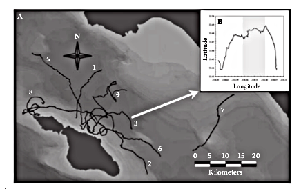
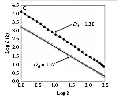
• The fine scale movement patterns of the ocean sunfish Mola mola (From Seuront 2009). The inset is the detail of the diurnal and nocturnal (shaded) movements.

  

Mola mola swimming

• The fractal dimension was calculated for diurnal and nocturnal movement paths and they were different.

  

• lower D during daylight suggest individuals move in more directed manner.

• Higher D In the night the movements were more complex suggesting individual interact with environmental heterogeneity on a finer scale.

• An increase in the complexity of spatial movements should indicate an increase in foraging or searching effort.

Characteristic features of fractals

• Mandelbrot Originally defined fractals as sets that have fractal dimension strictly greater than its topological dimension.

• There is no hard and fast definition but a list of properties.

• We refer to F as fractal if:

  1. F has a fine structure: i.e. detail on small scales.

  2. F is too irregular to be described by traditional geometrical language

  3. F has some form of self-similarity, perhaps approximate or statistical

  4. Usually the fractal dimension of F is greater than its topological dimension

Paper to read

1. Sugihara G, May RM (1990) Applications of fractals in ecology. Trends in Ecology & Evolution 5: 79–86.

Bibliography

• Gaedke U (1992) The size distribution of plankton biomass in a large lake and its seasonal variability. Limnology and Oceanography 37: 1202–1220.

• Seuront L (2009) Fractals and Multifractals in Ecology and Aquatic Sciences. Taylor & Francis.