Multifractals in ecology using R - Day 1
Posgraduate course, University of Maringá, 2013
Introduction to fractals and multifractals
What are fractals?
Highly irregular : fractal objects tend to be highly irregular and fill the space in which it is embedded.
Self-similarity : an object that displays the same basic pattern at all scales. The simplest fractals are deterministic, and are generated using recursive or iterative procedures.
Fractal Dimension : the characteristic are captured by a dimension that is a measure of complexity of the object.
Ecological fractals
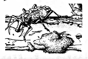
Fractal behavior can be observed looking at different scales. In the next figure (modified from Solé & Bascompte 2006) a beetle species walks on the surface of a trunk with lichens carrying lichens on its back.
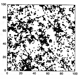
The spatial distribution of low canopy areas (less than 15m) in a rainforest in Panama (BCI) where clusters of many different sizes can be observed
Deterministic fractals
The Sierpinsky gasket : Starting with an equilateral triangle, the procedure consist on removing from the central portion an upside down equilateral triangle with half the side length of the starting triangle.
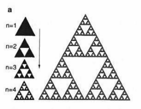
Deterministic fractals 1
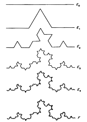
The Coch curve: A segment of length 1 is divided into thirds. The center one is replaced by the other two sides of an equilateral triangle of length 1/3.
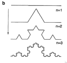
The curve occupies a definite space, but its length $L$ goes to infinity.
We can compute $L_n$ at different steps $n$
$L_0=1$
$L_1=4/3$
$L_2=(4/3)^2$
At an arbitrary step $L_n=(4/3)^n$ that goes to infinity as $n$ grows.
Why $L_n=(4/3)^n$ ?
Dynamic fractals
Cellular automata (CA) are discrete time, discrete space and discrete state dynamical models. We will consider a one dimensional CA with N sites. We can think that each site contains one individual of one species $S_i(t)$ for $i=1,…,N$
Each time step all elements are updated following a rule table:
$S_i(t+1) = \Phi \left( S_{i-1}(t),S_{i}(t),S_{i+1}(t) \right)$
The state of each unit change according to its own state and the state of some neighborhood.
The simplest case is that we have only one species: the possible states are 0 and 1.
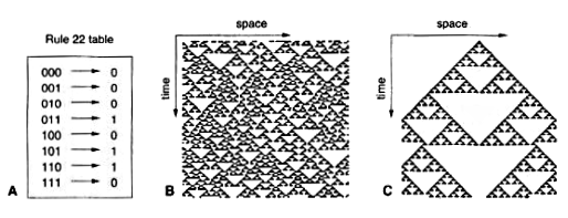
Exercise: play with 1D CA
Rule 22 (monogamy)
  current pattern     111   110    101    100    011    010   001   000
  -----------------  ----- -----  -----  -----  -----  ----- ----- -----
  new state            0     1      1      0      1      0     0     0
Starting with the following initial configurations
  a) 1 0 1 0 1 0 1 0 1 0

  b) 0 1 1 0 1 0 1 1 0 0
But the rule 22 does not generate the Sierpinsky triangle, the following rule generates it:
  current pattern    111   110   101   100   011   010   001   000
  ----------------- ----- ----- ----- ----- ----- ----- ----- -----
  new state           0     1     0     1     1     0     1     0
Starting with the following initial configurations
a) 0 0 0 0 1 0 0 0 0 0
Random Fractals
All the previous fractals constructions have random analogues. In the Von Koch curve we replace the middle third by the sides of an equilateral triangle, we might toss a coin to determine the position of the new part above or below the removed segment.
Statistical self similarity
The pattern of random fractals is self-similar in the statistical sense.
A given property $L(r)$, which can be length, mass, population abundance or number or species, measured at some scale of resolution $r$.
Then we look at a different scale $r’=\alpha r$. If $\alpha < 1$ then is a finer resolution, else a coarser resolution.
Statistical self similarity means that $L(r)$ is proportional to $L(\alpha r)$
$L(\alpha r) = k L(r)$
where k is a constant.
This definition implies that the statistical features of a fractal set are the same when measured at different scales.
Scaling laws
Statistical self similar patterns can be analyzed by power laws or scaling laws
Zipf’s law : one of the best known scaling laws
The fraction of cities $N(n)$ with $n$ inhabitants shows a power law dependence:
$N(n) \propto n^{-r}$ with $r \approx 2$
An example of an ecological scaling law is the frequency distribution of biomass, the plot shows the cumulative distribution $N(>n)$ against biomass
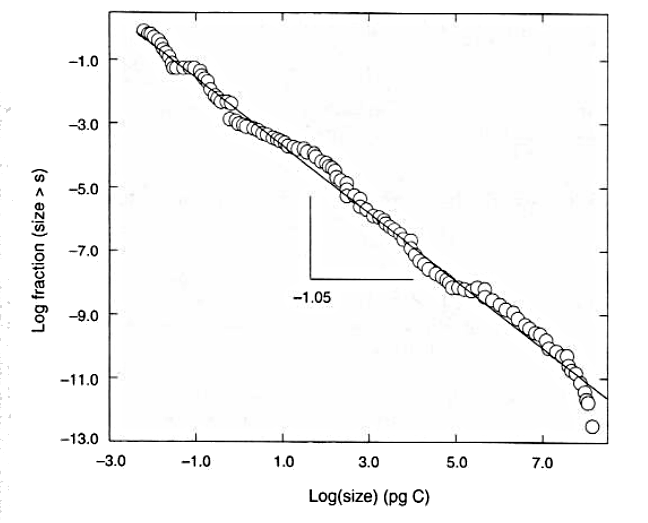
Scaling in the cumulative biomass distribution of all organisms in lake Konstanz (from Gaedke 1992).
For a scaling law $N(n) \propto n^{-r}$ we get $N(>n) \propto n^{-r+1}$
Power laws are scale invariant
To show that power laws are scale invariant we can see the effect of a scale transformation.
Self similarity implies:
$\frac{L(r)}{L(\alpha r)}=k$
Let us assume that $L(r)$ follows a power law
$L(r)=A r^\eta$
then
$\frac{A r^\eta}{A (\alpha r)^\eta} = \frac{1}{\alpha^\eta} = k $
Fractal dimension
Let us consider different geometric objects:
A line $\Omega_1$ of length $L$
A square $\Omega_2$ of area $L^2$
A cube $\Omega_3$ with volume $L^3$
We want to cover these with a set of identical non-overlaping segments/squares/cubes of side $\epsilon L$ with $\epsilon < 1$.
The number of segments required to cover $\Omega_1$ will be
$N(\epsilon) = \frac{L}{\epsilon L} =\epsilon^{-1}$
For the squares $\frac{L^2}{(\epsilon L)^2} =\epsilon^{-2}$
In general
$N(\epsilon) = \epsilon^{-d}$
Where $d=dim(\Omega_d)$
Fractal dimension 1
Thus we can define a dimension taking logarithms
\[d = -\lim_{\epsilon \to 0}\frac{\log N(\epsilon)}{\log \epsilon}\]Why we need the limits?
We can apply it to the Sierpinsky gasket:
For the first step we need 1 triangle of side $\epsilon_0=1$
For the second step we need $N_1(\epsilon)=3$ of side $\epsilon_1=1/2$
In general $N_n(\epsilon)=3^n$ triangles of side $\epsilon_n=(1/2)^n$
The fractal dimension
\[d = -\lim_{n\to \infty}\frac{\log 3^n}{\log (1/2)^n}=\frac{log 3}{log(1/2)}=1.5849\]This is a non-integrer value between a line dim=1 and a surface dim=2. In general fractal objects have a dimension below of the dimension of the space that contains it.
Exercise: what is the dimension of the Koch Curve
- $-\frac{log 4}{log(1/3)}$
Estimation of fractal dimension
How to compute fractal dimensions for natural objects that display statistical self similarity?
The box counting algorithm
We cover the object with square non-overlaping boxes of size $\epsilon^2$ and repeat the procedure using a range of $\epsilon$ values
This range will be limited by the resolution scale $\epsilon_m$ the pixels of our system, and the system size $\epsilon_M$
For each $\epsilon$ in our range the number of boxes $N_b(\epsilon)$ containing at least one part of the object will be counted
Following the definition of dimension we can see that $N_b$ will approximately scale as
$N_b(\epsilon) \thicksim \epsilon^{-d}$
in practice $d$ is estimated by the slope of the scaling relation
$-\log(N_b(\epsilon))/\log(\epsilon)$
An ecological example
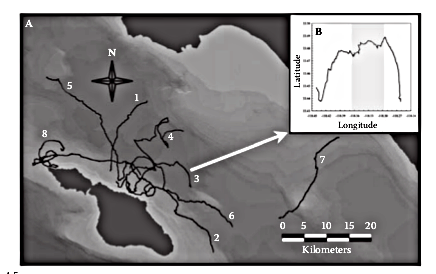
The fine scale movement patterns of the ocean sunfish Mola mola (From Seuront 2009). The inset is the detail of the diurnal and nocturnal (shaded) movements.
Mola mola swimming
The fractal dimension was calculated for diurnal and nocturnal movement paths and they were different.
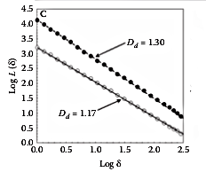
lower D during daylight suggest individuals move in more directed manner.
Higher D In the night the movements were more complex suggesting individual interact with environmental heterogeneity on a finer scale.
An increase in the complexity of spatial movements should indicate an increase in foraging or searching effort.
Characteristic features of fractals
Mandelbrot Originally defined fractals as sets that have fractal dimension strictly greater than its topological dimension.
There is no hard and fast definition but a list of properties.
We refer to F as fractal if:
F has a fine structure: i.e. detail on small scales.
F is too irregular to be described by traditional geometrical language
F has some form of self-similarity, perhaps approximate or statistical
Usually the fractal dimension of F is greater than its topological dimension
Paper to read
- Sugihara G, May RM (1990) Applications of fractals in ecology. Trends in Ecology & Evolution 5: 79–86.
Bibliography
Gaedke U (1992) The size distribution of plankton biomass in a large lake and its seasonal variability. Limnology and Oceanography 37: 1202–1220.
Seuront L (2009) Fractals and Multifractals in Ecology and Aquatic Sciences. Taylor & Francis.
