Using Infomap for Food Web Modularity

This post introduces how to calculate and assess modularity in food web networks using the multiweb R package. We illustrate this with the Potter Cove food web (included in the package as netData[[23]]) and show how to run Infomap, compare implementations, and apply network randomization routines. You need to install infomap

Infomap Installation

and ‘multiweb’

require(devtools)
install_github("lsaravia/multiweb")

Run Infomap on an Empirical Food Web

We use the run_infomap() function, an interface between R and the external Infomap binary:

library(multiweb)
library(tidyverse)

g <- netData[[23]] # Potter Cove food web

py_infomap0 <- run_infomap(g, output_dir = ".", return_df = TRUE)
py_infomap0$codelength

[1] 4.36376

To explore the module membership:

py_infomap0 <- py_infomap0$communities
py_infomap0 %>% filter(module == 1)

Output for module 1:

  module                       node      flow
1      1 Gobionotothen gibberifrons 0.0162264
2      1          Notothenia rossii 0.0593102
3      1     Harpagifer antarcticus 0.0411967
4      1  Lindbergichthys nudifrons 0.0255800
5      1    Chaenocephalus aceratus 0.1391530
6      1  Parachaenichthys charcoti 0.0024676

Alternatively, retrieve an igraph-compatible object:

py_infomap <- run_infomap(g)
py_infomap$codelength

IGRAPH clustering infomap, groups: 7, mod: 0.18
+ groups:
  $`1`
  [1] "Gobionotothen gibberifrons" "Notothenia rossii"          "Harpagifer antarcticus"     "Lindbergichthys nudifrons" 
  [5] "Chaenocephalus aceratus"    "Parachaenichthys charcoti" 


$codelength
[1] 4.36376

❗ A Note on cluster_infomap

The same algorithm is included in igraph as cluster_infomap(), but it produces different results:

ig_infomap <- cluster_infomap(g)
ig_infomap$codelength

IGRAPH clustering infomap, groups: 1, mod: 0
+ groups:
  $`1`
    [1] "Aged detritus"                "Polychaeta"                   "Polynoidae"                   "Gitanopsis squamosa"         
    [5] "Gobionotothen gibberifrons"   "Notothenia rossii"            "Ophionotus victoriae"         "Aequiyoldia eightsii"        
    [9] "Salpidae"                     "Gammaridea"                   "Ostracoda"                    "Oligochaeta"                 
  + ... omitted several groups/vertices


[1] 5.845473

We validated our results against the Infomap web interface and found that run_infomap() yields consistent and accurate results. We therefore recommend not using cluster_infomap() for empirical studies.

Randomizing Networks for Null Model Comparison

1. Curveball Randomization

We can randomize networks using the curveball algorithm, which preserves row/column sums (degree sequence):

gl <- curve_ball(g)
modl <- calc_modularity(gl, cluster_function = run_infomap)

Plotting the distribution of modularity across replicates:

ggplot(modl, aes(x = Modularity)) +
  geom_density(fill = "skyblue", alpha = 0.5) +
  geom_vline(xintercept = py_infomap$modularity, color = "red", linetype = "dashed") +
  labs(title = "Distribution of Modularity under Curveball Randomization",
       x = "Modularity", y = "Density") + theme_bw()

2. Degree-Preserving Shuffling

This routine preserves the in- and out-degree sequence via iterative edge swaps:

shuffle_network_deg(input_graph, delta = 10)

Where delta is the number of swaps

We use this in a more systematic way with:

result <– generate_shuffled_seq(
  netData[[29]], 
  max_delta= 1000,
  modularity_func = run_infomap, 
  shuffle_func = shuffle_network_deg
)

This produces a sequence of 1000 networks each with 10 edge swaps using the shuffle_network_deg algorithm

Plotting modularity over shuffle steps can help detect when modularity deviates from the empirical structure.

# Extract modularity metrics
metrics_df <- result$Metrics

# Add a column identifying the original vs shuffled
metrics_df$Type <- ifelse(metrics_df$Step == 1, "Original", "Shuffled")

# Plot modularity over shuffle steps
ggplot(metrics_df, aes(x = Step, y = Modularity, color = Type)) +
  geom_line() +
  geom_point(size = 2) +
  labs(title = "Modularity over Network Shuffling",
       x = "Shuffle Step",
       y = "Modularity",
       color = "Network Type") +
  theme_bw()

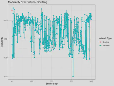
The graph shows that gradual shuffling runs through the distribution of modularity values ​​obtained by the shuffle_network_deg routine preserving in and out degree the same that curve_ball (previous graph). As shuffling proceeds, modularity explores a broad range of values spanning the distribution obtained from independently randomized networks (see previous figure). Across 1,000 iterations, no convergence or stabilization of modularity is observed, indicating that modular structure remains highly sensitive to the specific configuration of links generated at each shuffle step.

Summary

• run_infomap() wraps the external Infomap binary and gives reliable modularity estimates.
• cluster_infomap() (igraph) gives different results than the original app.
• Randomization routines like curve_ball() and shuffle_network_deg() help assess structural significance.
• shuffle_network_deg() is useful for increasingly randomize the network in steps but it is slower for a complete randomization.
• curve_ball() randomize the network in an efficient and unbiased way
• Visualizing modularity distributions is key for interpreting modular structure.

Resources

• 📦 multiweb GitHub Repository
• 📘 Infomap Installation
• 📄 Strona et al. 2014. Nature Communications 5:4114. https://doi.org/10.1038/ncomms5114

Feel free to reach out or open an issue on GitHub if you’d like to contribute!