Stochastic Network Interaction Model (SNIM) Tutorial

This is a beautifully simple ecological network model that can simulate predator-prey and competitive multispecies dynamics. This is the B model of the paper ¹, I read it long ago and for many years I wanted to make a version of it, finally, I did it.

You can find the source code here https://github.com/lsaravia/snim. To install it, clone the repository using git clone or download and compile it, following the instructions in the README.

The model description from ¹ is the following:

The second model again involves a set of S (possible) species plus empty sites (pseudospecies labelled 0). This set (the species pool) $\Omega(S)$ is then a discrete set:

$\Omega(S) = {0,1,2,…,S}$

where 0 indicates empty space, available to all species from the pool. Three basic types of transition are allowed to occur. Let us call $ A,B \in \Omega(S )$ two given spcies present at a given step. These possible transitions are summarized as follows.

(i) Immigration: an empty site is occupied by a species randomly chosen from the set of (non-empty) species, i.e. $A \in \Omega(S )-{0}$:

$0 \xrightarrow{u_i} A$

This occurs with a probability of colonization (of empty sites) $\mu_i$ . Notice that this colonization depends on the particular species.

(ii) Death: All occupied sites can become empty with some fixed probability $e_i$ :

$A \xrightarrow{e_i} 0$

(iii) Interaction: the same rule as in model A is used, but here the probability of success $P_{ij}$ is weighted by the coefficients of the interaction matrix. Here we use

$P_{ij} = \pi[\Omega_{ij} - \Omega_{ji}]$

where $\pi[x]=x$ when $x > 0$ and zero otherwise. This probability of an interaction occurring in the system between species $i$ and $j$ is a measure of the interaction strength linking interacting species.

Using SNIM from R

Once installed, you can easily run simulations from R.

First, the model requires two input files:

• A species parameter file (.par)
• A simulation parameter file (.cfg)

Example: Species Parameter File

# Model parameters example 
#
3 10000                  # 3 species, total habitat 10000
0.1 	0.1 	0.1      # Immigration vector
1 		1 		1        # Extinction vector
# Omega interaction matriz 
# Species 0 is empty space
# Species 1 Predator eats 2 and 3
# Species 2 has higher growth rate 
# Species 3 outcompete species 2 
0.0 0.0 0.0 0.0
0.0 0.0 3.0 2.0
4.0 0.0 0.0 0.0
2.0 0.0 0.5 0.0

Explanation:

• First line: Number of species and total habitat size.
• Second line: Immigration rates for each species.
• Third line: Extinction rates for each species.
• Following lines: Omega interaction matrix (including intrinsic growth rates and interactions).

Example: Simulation Parameter File

# Simulation parameters example 
#
rndSeed = 0				# 0 means a random rndSeed
nEvals  = 500           # number of time steps
tau     = 0.01          # Integration step
iniCond = 1000          # Initial condition of abundance of species 
                        # if only one number is specified all the species will have the same initial conditions

Running the Model from R

A set of R functions are included. First, set a global variable pointing to the SNIM binary. Then, run the simulation:

# Global path to the binary of SNIM model
#
snimBin <- "~/Dropbox/cpp/CaNew/snim/dist/Release/GNU-Linux/snim"

source("R/snim_functions.r")

out <- run_snim_plot("simul.cfg","model3.par","model.out")

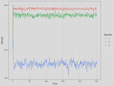
Animating the Dynamics with gganimate

An animation of the species densities can be created. First, set a shorter simulation (nEvals = 100), run the model again, and use:

require(gganimate)

ggplot(filter(out,Species!=0), aes(x = Time, y = Density,colour=Species)) + 
            geom_line() +  theme_bw() + scale_y_log10() + xlab("Years") + 
            transition_reveal(Time)

Have fun!