Overview
The multiweb package provides tools for analyzing and
comparing ecological networks, particularly food webs and multiplex
networks, through a set of reproducible and customizable functions. It
allows for the computation of structural and dynamic properties, module
detection, species roles, trophic positions, entropy- and
centrality-based metrics, structural stability thresholds, and
extinction simulations. Multiplex (multilayer) networks are supported
throughout, including aggregation, interactive visualization, and 3D
layer rendering.
This vignette introduces the general structure of the package and showcases typical usage patterns.
Data Structure
The multiweb package works with an individual network
and many functions accept lists of network objects,
where each network is typically a food web represented by a directed
graph. The preferred format is a list of igraph objects,
where each node is a species and directed edges represent trophic
links.
data("netData")  # A list of food web networks included in the package
net <- netData[[23]]
plot_troph_level_ggplot(net)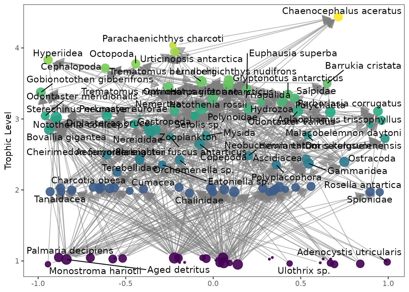
Basic Metrics
Global metrics
You can calculate a set of global network metrics such as number of species (S), connectance (C), mean trophic level using:
metrics_all <- calc_topological_indices(netData)
head(metrics_all)
#>              Network Size Top Basal  Omnivory Links       LD Connectance
#> 1             Angola   28   4     2 0.7500000   127 4.535714  0.16198980
#> 2         Baltic Sea   33   4     4 0.4848485   191 5.787879  0.17539027
#> 3 Barents Sea Arctic  159  43     7 0.5911950   848 5.333333  0.03354298
#> 4 Barents Sea Boreal  180  22     6 0.6722222  1546 8.588889  0.04771605
#> 5         Beach Peru   46  20     5 0.3043478    88 1.913043  0.04158790
#> 6     Beagle Channel  145  11    36 0.5517241  1115 7.689655  0.05303210
#>   PathLength Clustering Cannib   TLmean    TLmax  LOmnivory Components
#> 1   1.608333 0.35763293      3 2.897171 4.039211 0.21066115          1
#> 2   1.413115 0.30550459      7 2.393618 3.678314 0.12726540          1
#> 3   2.056762 0.16540420     10 2.843582 5.190582 0.15941579          1
#> 4   2.280036 0.24859772     23 3.002873 4.796090 0.22714502          1
#> 5   1.733032 0.09312639      0 2.633627 4.162698 0.07312069          1
#> 6   2.121089 0.22267298      0 2.376811 4.120973 0.22045506          1
#>   Vulnerability     VulSD Generality     GenSD
#> 1      5.291667 0.9515706   4.884615 0.5954786
#> 2      6.586207 0.7377881   6.586207 0.9311804
#> 3      7.310345 1.6540281   5.578947 1.0462268
#> 4      9.784810 1.2292073   8.885057 1.3645655
#> 5      3.384615 1.3800444   2.146341 0.8452183
#> 6      8.320896 1.2057445  10.229358 1.2296630
Modularity and Communities
Detect modules for a list of networks using any of the algorithms in igraph or Infomap (requires the installation of infomap in the system from https://www.mapequation.org/infomap/#Install). By default it uses the cluster_spinglass algorithm from igraph.
mod <- calc_modularity(netData,cluster_function = run_infomap)
mod$network_name <- names(netData)
head(mod)
#>   Modularity       network_name
#> 1 0.07638415             Angola
#> 2 0.05315096         Baltic Sea
#> 3 0.14248982 Barents Sea Arctic
#> 4 0.01091119 Barents Sea Boreal
#> 5 0.39617769         Beach Peru
#> 6 0.12863963     Beagle Channel
You can visualize the modular structure using:
mod  <- run_infomap(net)
plot_troph_level_ggplot(net, modules = TRUE, community_obj = mod)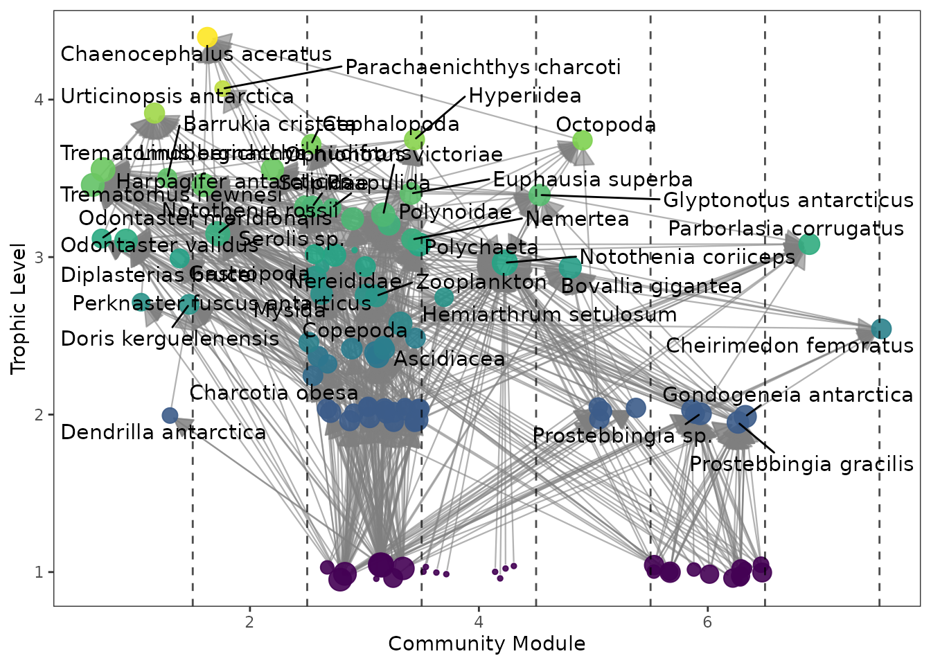
Topological Roles
You can compute species’ topological roles and plot them:
mod  <- run_infomap(net)
roles <- calc_topological_roles(net, community = mod)
roles_class <- classify_topological_roles(roles, net, community = mod)
head(roles_class$hub_conn)
#>   node            node_name   type within_module_degree among_module_conn
#> 1    7 Ophionotus victoriae modhub            2.9821909         0.1757812
#> 2   28     Benthic Diatomea modhub            2.8387437         0.3827160
#> 3   50       Fresh detritus modhub            2.9821909         0.4943311
#> 4    4  Gitanopsis squamosa modcon           -0.8893297         0.6875000
#> 5    6    Notothenia rossii modcon           -0.7369574         0.6603212
#> 6   10           Gammaridea modcon            0.5435892         0.6404959
roles_class$gp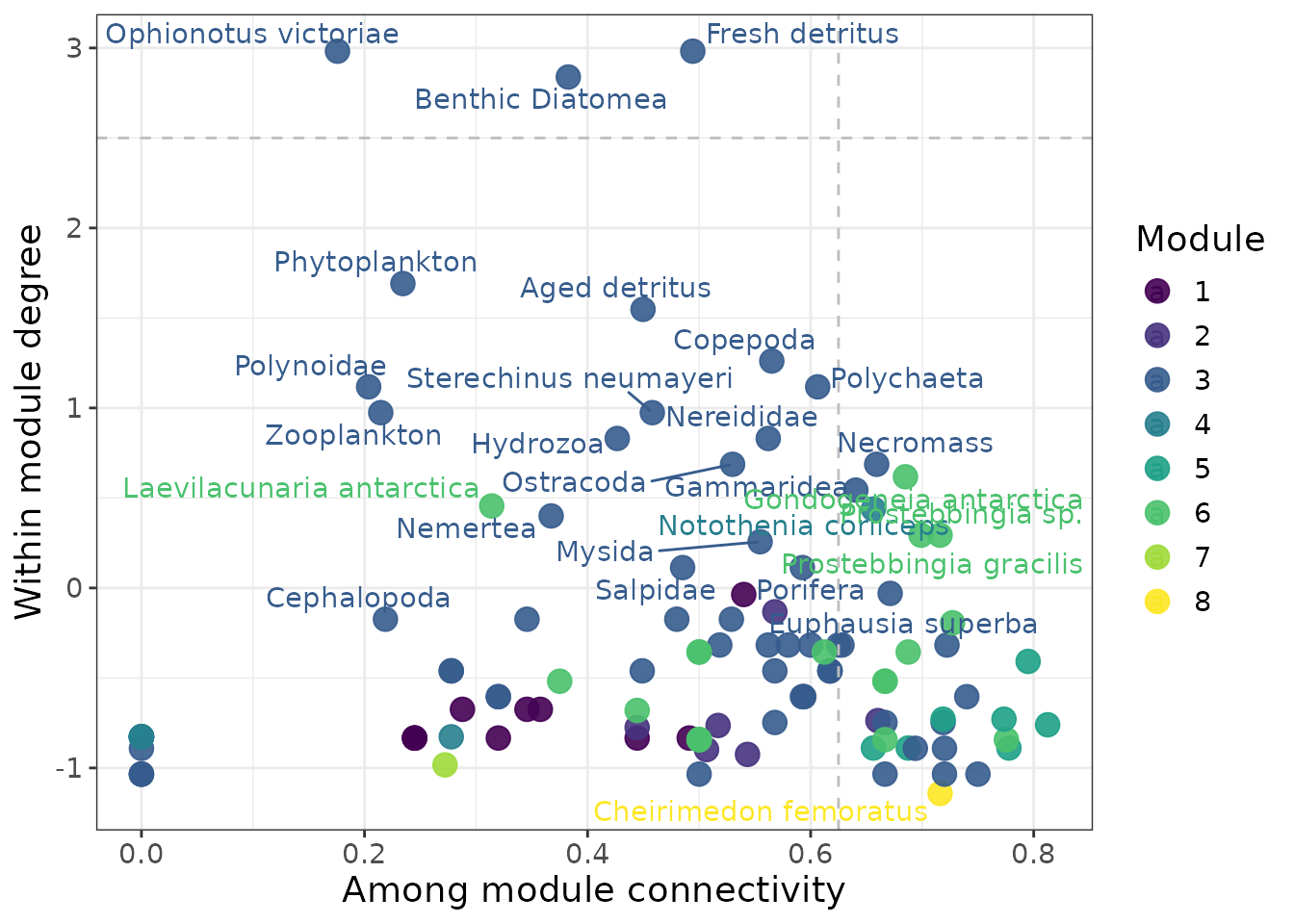
Entropy and Complexity
Quantify network complexity with singular value decomposition (SVD) entropy:
svd_ent <- calc_svd_entropy(net)
svd_ent
#> $Rank
#> [1] 56
#>
#> $Entropy
#> [1] 0.9092102
This metric is useful for comparing structural complexity across multiple networks.
Centrality measures
calc_centrality() generalizes centrality calculation to
any centrality function available in igraph (eigenvector
centrality, PageRank, betweenness, degree, etc.), returning both a
ranked table and a plot of the top species:
cent <- calc_centrality(net, centrality_func = igraph::page_rank)
head(cent$CentralityScores)
#> # A tibble: 6 × 2
#>   Species                 Centrality
#>   <chr>                        <dbl>
#> 1 Chaenocephalus aceratus     0.0976
#> 2 Urticinopsis antarctica     0.0976
#> 3 Notothenia coriiceps        0.0931
#> 4 Notothenia rossii           0.0397
#> 5 Trematomus bernacchii       0.0374
#> 6 Harpagifer antarcticus      0.0312
cent$Plot_Centrality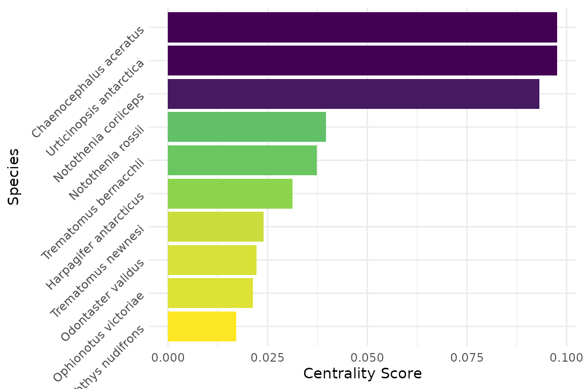
Detailed SVD importance
A more detailed decomposition of network complexity is available
through calc_svd_entropy_importance(), which — in addition
to entropy and rank — reports each species’ contribution to the dominant
singular value (i.e. its structural importance as prey and as
predator):
svd_imp <- calc_svd_entropy_importance(net)
svd_imp$Entropy
#> [1] 0.9092102
svd_imp$Plot_Prey_Importance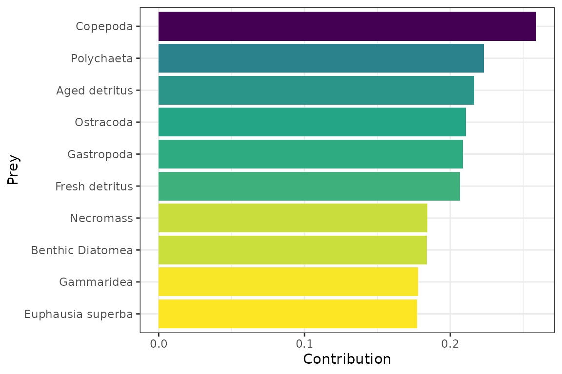
Randomizations and Null Models
The package includes tools for generating null models maintaining the degree distribution (Curbe ball algorithm):
rand_net <- curve_ball(net)
rand_metrics <- calc_modularity(rand_net, cluster_function = cluster_walktrap)

# Example: show distribution of connectance (C) and empirical value
library(ggplot2)
empirical_m <- calc_modularity(net, cluster_function = cluster_walktrap)$Modularity
ggplot(rand_metrics, aes(x = Modularity)) +
  geom_density(fill = "grey", color = "black") +
  geom_vline(xintercept = empirical_m, color = "salmon", linetype = "dashed", linewidth = 1) +
  theme_bw() +
  labs(title = "Distribution of Modularity in Randomized Networks",
       x = "Modularity")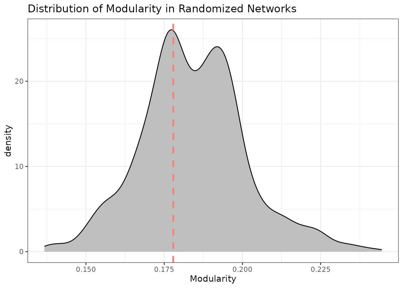
or using the niche model to generate random networks with the same size and connectance:
S <- metrics_all[23,"Size"]
C <- metrics_all[23,"Connectance"]
rand_net <- generate_niche(S,C,nsim=1000)
rand_metrics <- calc_modularity(rand_net, cluster_function = cluster_walktrap)

# Example: show distribution of connectance (C) and empirical value
library(ggplot2)
empirical_m <- calc_modularity(net, cluster_function = cluster_walktrap)$Modularity
ggplot(rand_metrics, aes(x = Modularity)) +
  geom_density(fill = "grey", color = "black") +
  geom_vline(xintercept = empirical_m, color = "salmon", linetype = "dashed", linewidth = 1) +
  theme_bw() +
  labs(title = "Distribution of Modularity in Randomized Networks",
       x = "Modularity")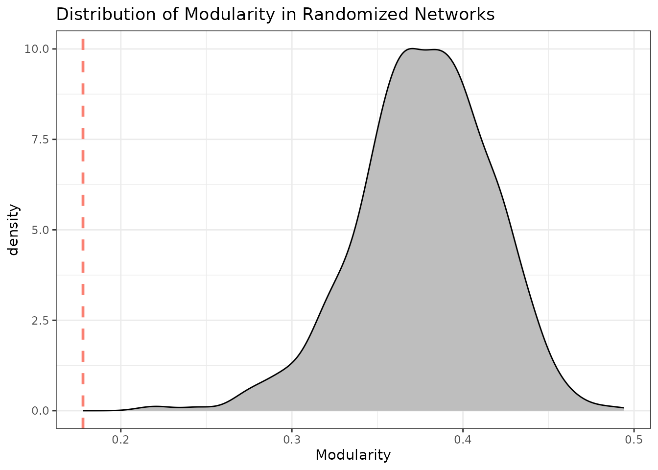
You can then use these null models to assess the significance of observed metrics.
Calculation of interaction intensity and weighted metrics
Here we calculate interaction intensity using body mass and density data from the Potter Cove food web (data included in the package) and estimate weighted topological indices.
pc_i <- calc_interaction_intensity(
  PotterCove_bm,
  res_mm = r_bodymass,
  res_den = r_density,
  con_mm = c_bodymass,
  int_dim = D
)

# Build igraph object with weights from interaction strengths
g <- graph_from_data_frame(
  d = pc_i %>% dplyr::select(resource, consumer, weight = qRC),
  directed = TRUE
)

# Now compute weighted indices
calc_weighted_topological_indices(g)
#>        wLD wConnectance  wTLmean   wTLmax wLOmnivory wVulnerability  wVulSD
#> 1 9.061722   0.08237929 2.015625 3.763807 0.07262355       12.25968 4.99523
#>   wGenerality   wGenSD
#> 1    5.863761 3.124224
Alternative interaction intensity estimation (O’Gorman 2010)
As an alternative to the body-mass/density approach above — useful
when resource density data are unavailable —
calc_interaction_intensity2() estimates interaction
strength from predator body mass and the number of resources per
consumer, following O’Gorman et al. (2010):
edge_list <- tibble::tibble(
  predator = c("A", "A", "B", "C"),
  prey = c("B", "C", "D", "D"),
  predator_mass = c(10, 10, 5, 3)
)

calc_interaction_intensity2(
  edge_list,
  consumer_n = predator,
  resource_n = prey,
  bodymass_n = predator_mass,
  output_format = "edgelist"
)
#> # A tibble: 4 × 3
#>   predator prey      qRC
#>   <chr>    <chr>   <dbl>
#> 1 A        B     0.00281
#> 2 A        C     0.00281
#> 3 B        D     0.00669
#> 4 C        D     0.00760
Using multiplex networks
The package also supports multiplex networks, where multiple types of interactions are represented as layers. You can create a multiplex object and compute metrics across layers.
fpath <- system.file("extdata", package = "multiweb")
dn <- list.files(fpath,pattern = "^Kefi2015.*\\.txt$")
mnet <- readMultiplex(dn,c("Negative","Positive","Antagonistic"),fpath,skipColum=2)
You can then compute metrics like modularity for the entire multiplex structure, in this case using the interface to info_map algorithm.
mod_multi <- run_infomap_multi(mnet)
head(mod_multi$communities)
#>   module                   node layer        flow
#> 1      6     acanthocyclus gayi     1 0.002427980
#> 2      6 acanthocyclus hassleri     1 0.002413950
#> 3      7       chiton  granosus     1 0.000546136
#> 4      7    fissurella  costata     1 0.000000000
#> 5      7     fissurella  crassa     1 0.000615915
#> 6      7    fissurella  limbata     1 0.000000000

plots <- plot_multiplex_modules(mnet, mod_multi$communities)
cowplot::plot_grid(plotlist = plots, ncol = 3)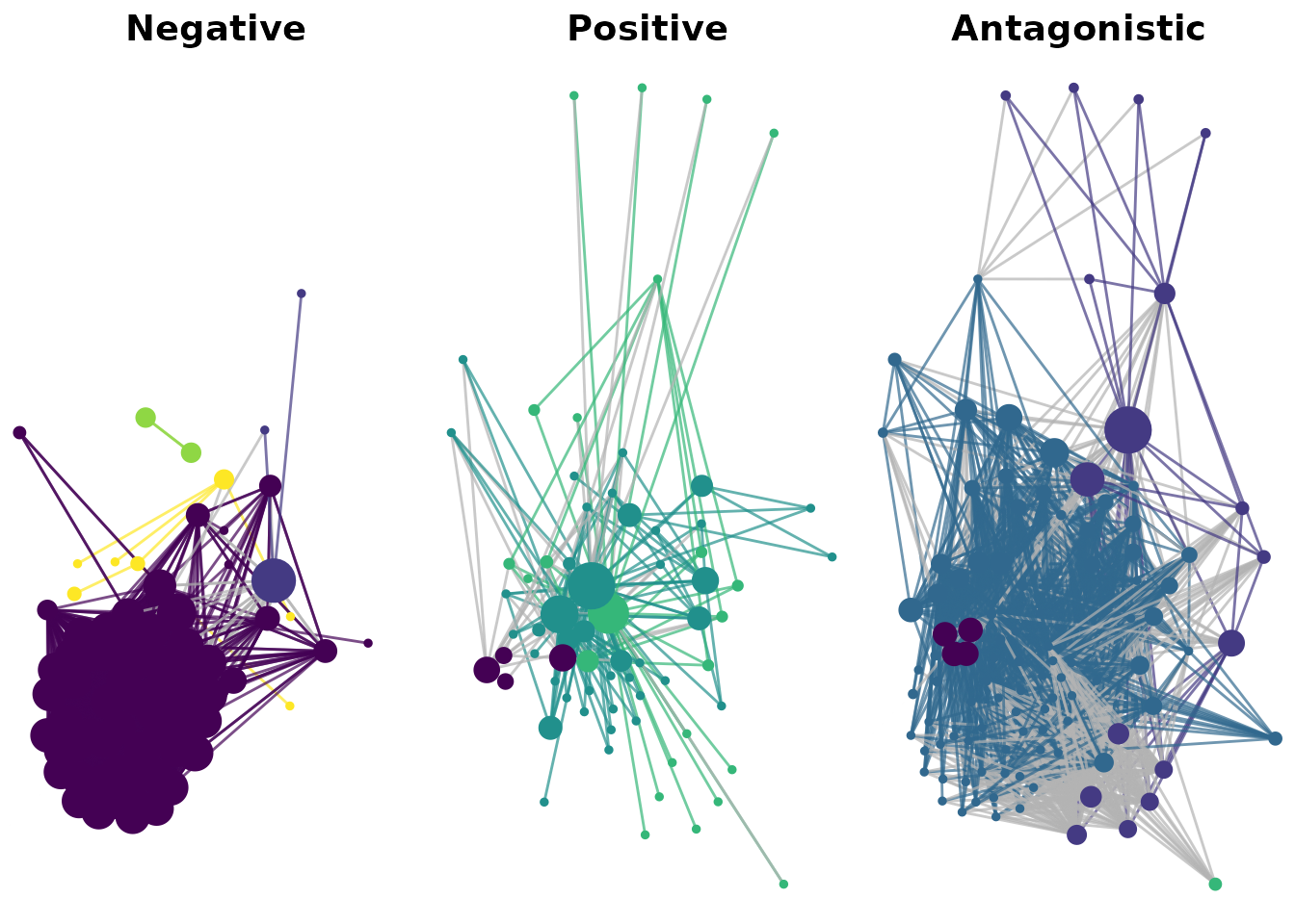
Layers sharing the same node set can be combined into a single
aggregate network — summing edge weights where interactions coincide
across layers — which is useful as a common backbone for layout or as an
approximation of overall interaction load.
harmonize_node_sets() first ensures every layer shares the
same set of nodes (adding isolated nodes where needed) before
aggregating:
mnet_named <- mnet
names(mnet_named) <- c("Negative", "Positive", "Trophic")
mnet_named <- harmonize_node_sets(mnet_named)
agg_net <- aggregate_multiplex_network(mnet_named)
agg_net
#> IGRAPH 33c480c DNW- 106 4554 --
#> + attr: name (v/c), weight (e/n)
#> + edges from 33c480c (vertex names):
#>  [1] acanthina monodon ->concholepas concholepas
#>  [2] acanthina monodon ->corallina offcinalis var. chilensis
#>  [3] acanthina monodon ->gelidium spp.
#>  [4] acanthina monodon ->gulls
#>  [5] acanthina monodon ->heliaster helianthus
#>  [6] acanthina monodon ->perumytilus purpuratus
#>  [7] acanthina monodon ->semimytilus algosus
#>  [8] acanthocyclus gayi->acanthocyclus gayi
#> + ... omitted several edges
For a 3D view of all layers stacked together,
plot_multi3D() (adapted from the muxViz
project) renders each layer as a semi-transparent plane using
rgl, optionally with an aggregate layer on top. This opens
an interactive OpenGL device, so it is best explored in an active R
session rather than rendered here:
plot_multi3D(
  g.list = mnet_named,
  layer.colors = RColorBrewer::brewer.pal(3, "Set2"),
  node.colors = "auto",
  node.size.scale = 0.5,
  show.aggregate = TRUE
)
Structural Stability (QSS)
Estimating the stability threshold
Real food webs must be dynamically stable, which requires some
minimal level of intraspecific self-regulation (self-damping). Because
the true amount of self-regulation is rarely known,
calc_stability_threshold() searches for the
selfDamping value at which a target proportion of simulated
community matrices (Jacobians) become unstable — by default, 5%
negative-eigenvalue crossings — using [calc_QSS()] internally. Lower
(more negative) thresholds indicate networks that require less
self-regulation to remain stable:
stab <- calc_stability_threshold(net, nsim = 200, ncores = 1, verbose = FALSE)
stab$threshold
#> [1] -9.083333
The search trajectory can be visualized directly:
plot_stability_curve(stab)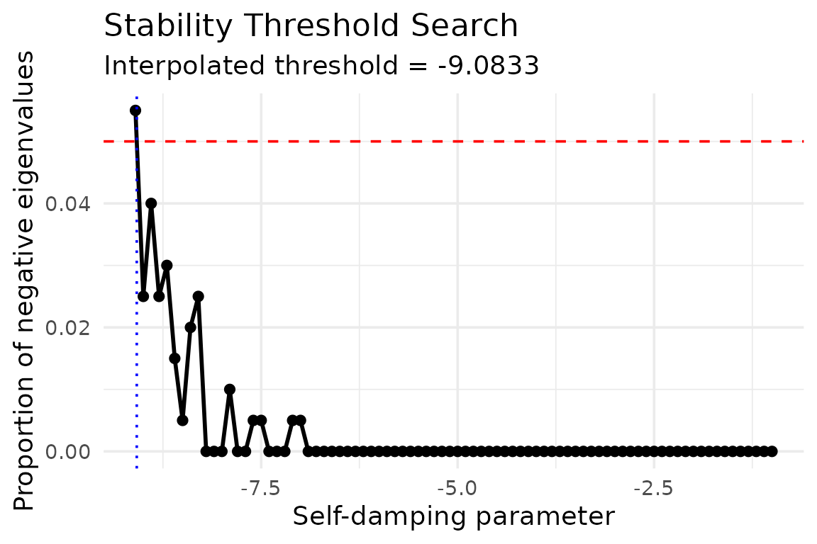
Extinction simulations
multiweb also provides tools to evaluate how the loss of
one or more species affects structural stability, by comparing QSS
distributions before and after deletion — useful for identifying
keystone species or estimating robustness to targeted or random
extinctions.
To compare the whole network against the network without a given set of species:
sp_sample <- V(net)$name[1:3]
ext_grp <- calc_QSS_extinction_dif_grp(net, sp_sample, nsim = 100, ncores = 1)
head(ext_grp)
#>   Size Connectance Components  QSS_all  QSS_ext     difQSS
#> 1  107  0.05074679          1 3.606543 3.309827  0.2967167
#> 2  107  0.05074679          1 4.015366 3.319860  0.6955062
#> 3  107  0.05074679          1 3.977981 3.507072  0.4709096
#> 4  107  0.05074679          1 3.557852 3.022157  0.5356952
#> 5  107  0.05074679          1 4.824300 4.317341  0.5069594
#> 6  107  0.05074679          1 3.681747 4.844631 -1.1628837
To simulate an incremental extinction sequence (species removed one at a time, without secondary extinctions):
ext_seq <- calc_QSS_extinctions_seq(net, sp_sample, nsim = 100, ncores = 1)
head(ext_seq)
#>      maxre Size Connectance Components Last_deleted
#> 1 3.947036  110  0.05363636          1        Total
#> 2 3.317002  110  0.05363636          1        Total
#> 3 3.480043  110  0.05363636          1        Total
#> 4 4.502018  110  0.05363636          1        Total
#> 5 3.224644  110  0.05363636          1        Total
#> 6 3.670907  110  0.05363636          1        Total
Note: nsim and ncores are set low here for
a fast-running vignette; for actual analyses, larger nsim
(e.g. 1000) and more cores are recommended for stable estimates.
Interactive Visualization
For exploratory work, multiweb provides interactive,
draggable network visualizations built on visNetwork, as an
alternative to the static ggplot2/ggraph plots
shown above. Nodes are still organized by trophic level on the y-axis,
but can be dragged, zoomed, searched, and hovered for details.
plot_troph_level_visNet(net, modules = TRUE)For multiplex networks, plot_troph_level_visNet_multi()
overlays all interaction layers on the same trophic-level plot,
computing trophic level only from the designated trophic layer, with
distinguishable edge colors/styles per layer, an interactive layer
filter, and a legend:
plot_troph_level_visNet_multi(
  mnet_named,
  trophic_layer = "Trophic",
  layer_dashed = c("Negative", "Positive")
)
Note: when knitting to HTML these render as interactive embedded widgets; if the vignette is exported to PDF for external documentation (e.g. as supporting material), interactivity will be lost and a static screenshot may be preferable.